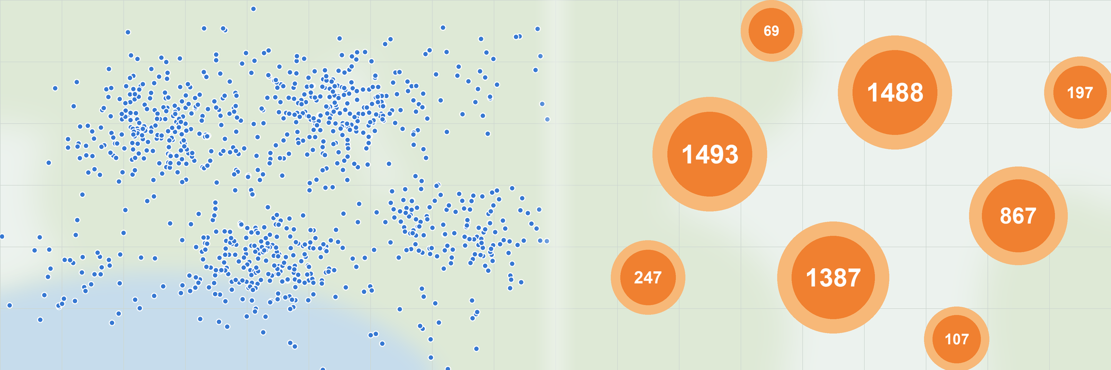
Book Corners has grown quite a lot since I introduced it earlier this year. Today it has 37,238 approved public bookcases, and the map is the page people use the most. A few days ago I looked at how much data the map endpoint was sending and I didn’t like what I found.

The problem

The map page loads its markers from a GeoJSON endpoint: /map/libraries.geojson. The page always sends the current zoom level and the visible area (the “bounds”), and at low zoom levels the server already groups libraries into clusters using PostGIS.

That works fine for the map page itself, but there were a few cases where the endpoint returned one feature for every single library:

• requests without any parameter (direct calls, old links, bots…)
• requests with a zoom but without bounds
• requests with invalid bounds, which silently fell back to the full dataset
• any search filter (keywords, city, country, postal code), which turned clustering off at every zoom level

These are the numbers I measured in production:

On top of that, the full response was serialized and stored in the database cache every 5 minutes, or every time a library was edited. A search for “Germany” from the world view was sending 5,235 pins to the browser, which then had to cluster them again on the client side.

Clustering with ST_SnapToGrid

Server-side clustering was already in place for unfiltered requests. The idea is simple: PostGIS ST_SnapToGrid snaps every point to a grid whose cell size depends on the zoom level (40 degrees at zoom 0, 0.1 degrees at zoom 11), and then I group by the snapped point. Each group becomes a single cluster feature with a count, a centroid and the bounding box of its points, so the client can zoom to it when you click it.

The limitation was that the SQL query was written by hand and only knew how to filter by status = 'approved' and by bounds. Search filters live in the Django ORM (full text search, icontains, iexact…) and I really didn’t want to duplicate all of them in raw SQL.

Using the ORM queryset as a subquery

The solution I found is to let Django compile the filtered queryset and use it as a subquery in the clustering SQL. This way every search filter goes through exactly the same code used by the list view and the individual pins:

 1
 2
 3
 4
 5
 6
 7
 8
 9
10
11
12
13
14
15
16
17
18
19
20
21
22
23
24
25
26
27
28
29
30
31

def build_clustered_features(
    *,
    zoom: int,
    bounds: Polygon | None = None,
    queryset: QuerySet[Library] | None = None,
) -> list[dict[str, object]]:
    grid_size = get_grid_size_for_zoom(zoom)

    if queryset is None:
        queryset = Library.objects.filter(status=Library.Status.APPROVED)
    if bounds is not None:
        queryset = queryset.filter(location__within=bounds)

    inner_sql, inner_params = (
        queryset.order_by().values("location", "city", "country").query.sql_with_params()
    )

    sql = f"""
        SELECT
            ST_X(ST_Centroid(ST_Collect(location))) AS lng,
            ST_Y(ST_Centroid(ST_Collect(location))) AS lat,
            COUNT(*) AS point_count,
            MIN(city) AS sample_city,
            MIN(country) AS sample_country,
            ST_Extent(location) AS extent
        FROM ({inner_sql}) AS filtered_libraries
        GROUP BY ST_SnapToGrid(location, %s)
        ORDER BY point_count DESC
    """
    params = [*inner_params, grid_size]
    ...

A couple of details are worth mentioning:

• order_by() with no arguments removes the ordering, which would be useless (and slower) inside a subquery. The full text search, for example, orders by rank.
• values() keeps the subquery small: the clustering only needs the location, the city and the country.
• sql_with_params() returns the parameters separately, so the user input is still passed safely to the database driver and never formatted into the SQL string.

Proximity searches (“near Berlin”) are the only exception: they already re-center the map at zoom 12 and are limited by a radius, so they keep returning individual pins.

Caching and counts

Clustered responses are cached, and the cache key now includes a hash of the filter values. Without it, a search for Germany could have been served the clusters cached for Italy. The key also includes a version number which is increased every time a library changes, so an edit or an approval invalidates every cached cluster response at once.

I also had to be careful with the counts. The map shows a summary like “Showing 86 of 5235 libraries on the map”: the first number is how many libraries are in the visible area and the second one is the total for the current search. Clustered responses keep exactly the same meaning, so the text is still correct when you look at clusters instead of pins.

Requests without bounds

The last change was about requests without bounds. My first version capped their zoom at 11, the last zoom level with clustering. When I checked production after deploying, I noticed that ?zoom=13 without bounds was still returning 12,203 clusters and 3.16 MB: a grid of 0.1 degrees over the whole world is still a lot of cells!

A request without bounds is a request for the whole world, so now it always uses the zoom 0 grid, whatever zoom it sends. The map page always sends bounds, so users don’t notice any difference.

Results

These are the numbers measured in production after the three changes were deployed:

The last row is there to show that nothing was lost: when you are zoomed into a city you still get individual pins, with their popups.

I also checked the real map in a browser. I searched for Germany and kept clicking the first cluster until the pins appeared:

The first click shows 817 libraries and not 1,493 because zooming in leaves part of that cluster outside the visible area, and the summary only counts what you can see.

Conclusion

The worst case went from 13.85 MB to 6.7 KB, and a country search from the world view went from 1.9 MB to less than 500 bytes. The most useful part, in my opinion, was reusing the Django queryset as a subquery: it let me cluster any search without writing a single filter twice.

If you want to see it in action, go to the Book Corners map, search for your country and start clicking on the clusters.